|
Optimization of seam
annealing process
with the help of 2D simulations
John Inge Asperheim and
Leif Markegård
EFD Induction a.s |
Introduction
In the production of welded pipes
according to API standards, a normalization of the weld and heat
affected zone (HAZ) is required. The weld of thick-walled tubes shows an
hour-glass shaped HAZ caused by the ”corner effect” in the weld Vee. The
microstructure, particularly at the external and internal surfaces, is
very coarse-grained. The aim for the heat treatment is to reestablish a
homogeneous and fine-grained microstructure in the HAZ.
To achieve a fine-grained
microstructure after the normalization, it is important to limit the
temperature on the external surface of the pipe, which is closest to the
coil, to avoid grain re-growth, and to reach high enough austenitisation
temperature in a sufficiently wide zone at the inner surface. The width
at the inner surface must cover the width of the HAZ, which has its
maximums at the surfaces, and the positioning tolerance of the heat zone
to the weld.
Even if low frequency is used for the
reheating of the weld zone, the heat penetration through the pipe wall
is partly reliant on heat conduction. Time needed for temperature
equalization through heat conduction increases proportionally to the
square of the wall thickness. The preferred welding method is by
induction, which requires higher minimum welding speed (minimum 10 – 12
m/min) than contact welding (minimum 5 – 6 m/min). One complication with
in-line normalizing heat treatment of thick-walled pipes is that the
heating requires considerable length in a line. This is due to the time
needed for temperature equalization through the pipe wall and the
required line speed. An important design work is to optimize the
temperature distribution in the heat zone and establish the minimum
heating length required. A 2D simulation, using coupled electromagnetic
and transient thermal calculations in a cross-section of the weld as it
passes through the different heating zones, is today an indispensable
tool. It is important to have good representations of the very nonlinear
and temperature dependant electrical and physical properties of the
steel, as well as heat losses by convection and radiation from the
surfaces and residual heat from the welding.
The maximum temperature limit as well
as the required minimum austenitisation temperature is dependent on
actual steel quality and required microstructure. The time at maximum
temperature for the surface close to the coil is from a few seconds up
to a few tens of seconds. Steel used in pipes that are produced
according to API standards normally contains alloy elements that resist
or slow down grain growth. One such element is aluminum, in the form of
fine aluminum nitride particles, that remain un-dissolved up to a
certain temperature. Above this temperature, often referred to as grain
coarsening temperature, the speed of grain growth increases rapidly.
Other alloy elements that slow down grain growth are vanadium, titanium
and niobium [1]. In our calculations we have used 1100ºC as maximum
temperature and 900ºC as required minimum austenitisation temperature.
In a production line the external
surface is accessible for temperature measurements, but the internal
temperature can only be judged through metallurgical examination of the
obtained microstructure (off-line check). The simulation results,
therefore, are also helpful in gaining a view of the temperature
distribution through the pipe wall and taking the right measures in case
of unacceptable results. Normally in a line, the
surface temperature in the center of the heated zone is used to regulate
the power to prevent overheating of the steel.
Normalization is defined as heating
to austenitisation temperature and cooling in still air. This is not the
case for seam normalizing as the colder part of the pipe acts as a
heat-sink and the temperature slope after heating is, first of all, a
result of the internal heat conduction in the pipe. The rather fast
cooling obtained, however, can be beneficial in producing a fine-grained
microstructure. To limit the length of the line one wants to start the
final water-cooling as early as possible. It is, however, important that
the transformation of the austenite be finalized. If the austenite is
retained at the point of water cooling, it results in quenched
microstructure as martensite. This normally is not allowed, at least not
as un-tempered martensite. The ITT (Iso-Temperature-Transformation) and
CCT (Constant-Cooling-Transformation) diagrams of the materials in
question and the calculated cooling curve are helpful tools in designing
the cooling part of the process.
The Model
We have represented the
process by a 2D cross-section of the tube and coil. In the real process
the tube moves through the production line and passes underneath a row
of seam annealing coils. By turning the power on and off it is possible
to simulate this movement. In order to reduce the number of computations
in sequence, we have left out the space between the coils in the study
on coil design. We have, therefore, computed on 3 equivalent sections
and the final cooling after the seam annealing section. The symmetry of
the geometry allows us to model only half the problem. We have used the
software Flux 2D. The layout of the model with a classical seam
annealing coil is shown in figure 1.
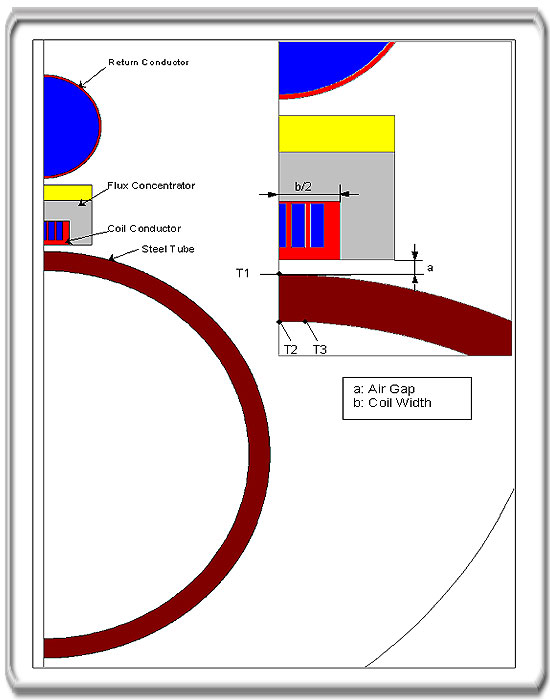
Figure 1. Computation domain
In the computations only
the tube itself and the surface regions that enable heat exchange from
the tube to the surroundings are included in the thermal part of the
problem. For the regions not included in the thermal part, the
representations of the material properties are simpler. Except for the
magnetic properties of the coil core, they are all constant. The
property assigned to the tube is the same throughout the computations,
but properties for the tube surface can be changed to represent
different cooling conditions.
When the tube arrives at
the first annealing coil, there is a temperature distribution in the
tube wall from the welding process that depends on the speed of the
line, the distance from welder to the first annealing and often water
cooling applied to allow ultrasonic inspection of the weld. The high
temperatures from the welding process are limited to a rather small mass
and even out quite fast [2]. Just as important is the heat generated in
the tube by the current going around the tube underneath the induction
welding coil. In the calculations on coil design presented in this
paper, we have started the computations with an elevated temperature of
200 °C in the entire tube. This temperature is calculated on the basis
of data we have from welders in mills running similar sized tubes.
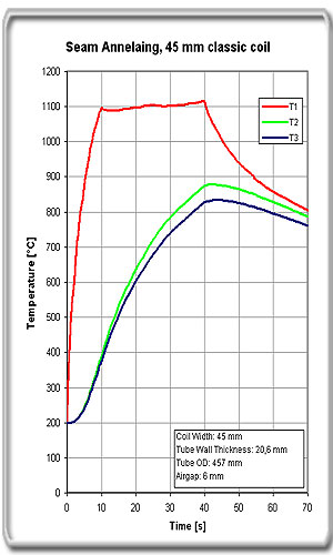
In the presentation of
the results, we have used three reference points for temperature
measurement. These can be seen in figure 1. Temperatures T1 and T2 are
at the symmetry line in the centre of the tube, T1 on the outer surface
and T2 on the inner surface. The point for temperature measurement T3 is
on the inner surface 10 mm from the symmetry axis.
Measurements
To verify that our
computations are reliable, we have taken some measurements with our
profiled coil. In this test we split one tube along its length to get
two half pipes. This made the inner surface of the tube more accessible
for temperature measurements. A setup like this is slightly different
from an actual mill. Computations, therefore, have been done on the same
“half pipe” setup. We have used material property data for steel 35CD4
(35CrMo4, AISI 4135) because good data is available for this particular
steel and the steel used in the tests, FeE 255, has properties close to
35CD4.
There were several
factors influencing the accuracy of the measurements in this test. Due
to the thermal expansion in the heated zone, the tube will bend when it
is heated. Since we used halves of a tube, the tube’s rigidity was
severely weakened. This allowed the tube to bend much more than it would
in an actual mill and resulted in some movement of the tube during
heating and, therefore, inaccuracy in the position of the thermocouples.
Temperature measurements were taken on a cross-section at the middle
point of the coil. When the tube was heated, we allowed it to bend away
from the coil at the ends. At the same time we placed insulating
material between coil and tube at the mid point to ensure that the
distance between the two remained acceptably constant at this point.
Temperatures are
measured with thermocouples, type K, welded on the inner and outer
surface at distances from the centerline of the tube’s heated zone. The
three points representing the temperatures from the computations (T1 –
T3) are presented in figure 2.
|
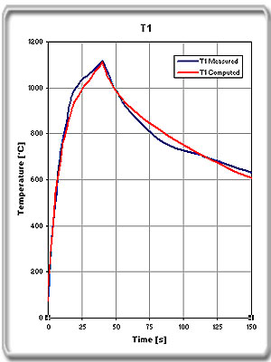
Figure
2a. T1 |
|
The tube had a
temperature of 75 °C at power on. The computation for direct
comparison with the measurements was started at the same
temperature.
When we compare calculated and measured temperatures, we see
that the measured values are generally a few degrees higher.
This can be explained as inaccuracy in current measurement or
air gap.
Data:
OD Tube: 327 mm
Wall Thickness: 17 mm
Air Gap: 6 mm
Coil Current: 9700 A
Frequency: 1450 Hz |
|
|
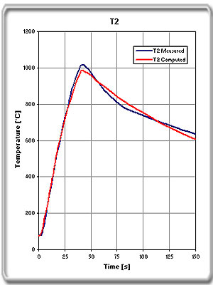
Figure
2b. T2 |
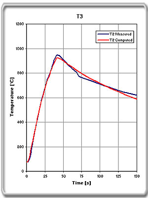
Figure
2c. T3 |
|
|
|
|
|
The tube had a
temperature of 75 °C at power on. The computation for direct comparison
with the measurements was started at the same temperature.
When we compare
calculated and measured temperatures, we see that the measured values
are generally a few degrees higher. This can be explained as inaccuracy
in current measurement or air gap.
Data:
OD Tube: 327 mm
Wall Thickness: 17 mm
Air Gap: 6 mm
Coil Current: 9700 A
Frequency: 1450 Hz
The specific heat value v.s. temperature have during
heating a hunch around 730 – 800 °C due to the energy required to
transform the material to austenite. In our calculation, the same
specific heat value v.s. temperature is
used during cooling. In reality the transformation energy
is released at lower temperatures as the transformation from austenite
takes place at lower and cooling-rate-dependant temperatures. This
simplification in representation of material properties is visible in
the curves during cooling. For our purposes, we can conclude that there
is good conformity since we are looking at cooling until transformation
is completed. At this point, all the transformation energy is released.
Coil design
When the coil is narrow compared with
the wall thickness, the heated zone has a shape that resembles a
half-cylinder. The heatflow lines, that are perpendicular to the iso-temperature
lines, bends tangential close to the inner surface. A narrow coil,
therefore, requires longer heating time (zone length) than a wider coil,
where the heatflow has a more radial direction in the required zone
width at the inner surface.
Table 1: Temperature scale for
T-color shade plots
|
 |
160 – 220
220 – 280
280 – 340
340 – 400 |
 |
400 – 460
460 – 520
520 – 580
580 – 640 |
 |
640 – 700
700 – 760
760 – 820
820 – 880 |
 |
880 – 940
940 – 1000
1000 –1060
1060 –1120 |
|
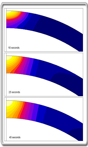
Figure 3a. T-colour shade plots
For 45 mm classic coil
|
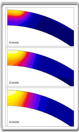
Figure 3b. T-colour shade plots
For 60 mm EFD Profiled Coil
|
|
 |
 |
|
Figure 4a.
Temperature vs. time plots
for 45 mm classic coil |
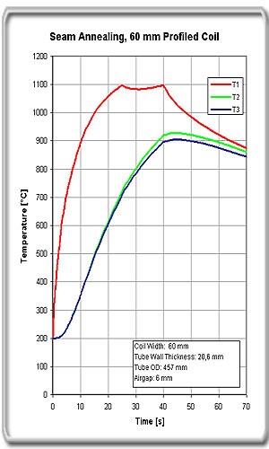
Figure 4b.
Temperature vs. time plots
for 60 mm EFD profiled coil |
When the material passes
Curie-temperature, a non-magnetic ”channel” is formed by the amount of
material that has exceeded the Curie-temperature. The shape of this
”channel”, or zone, determines the current distribution during the time
when this ”channel” is expanding. It is possible to optimize the heated
zone by adapting the coil profile and coil width.
With an increase in the coil width from 45 mm to 60 mm on
wall-thickness 20,6 mm, the required power increases about 14%. The
increase in power is less than the increase in coil width because, for
the wider coil, the zone length can be shorter resulting in a shorter
heating time. With longer heating time, the zone width is widened due to
heat conduction into the pipe.
Normally one type of coil must cover a range of wall
thicknesses. Coils with sufficient width to heat the largest wall
thickness at minimized heating zone length create a wider zone and
require more power than necessary for the smaller wall thickness range.
A wider heated zone gives better temperature homogeneity, which may also
lower the maximum temperature for smaller wall thicknesses. The zone
width also influences the temperature curve’s slope during cooling down
after the heating.
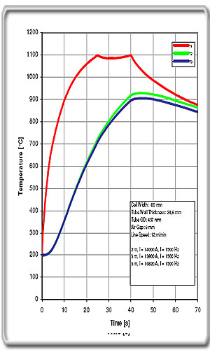
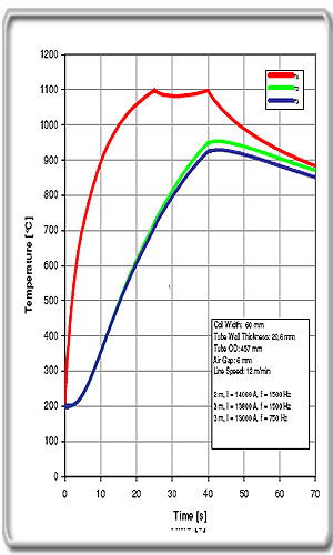
Frequency
We have made a comparison where the two first heating
zones of 2 m and 3 m are run at equal conditions in both cases at a
frequency of 1,5 kHz. In the first case the third zone has a frequency
of 1,5 kHz and in the second case 0,75 kHz. We see that the temperature
difference ∆T = T1 –T3 drops from 193 °C in the first case to 169 °C in
the second case. The conclusion is as expected, a lower frequency
improves the temperature homogeneity. A lower frequency, therefore,
makes it possible to get more power into the tube without exceeding the
maximum temperature at the surface. Another aspect of lowering the
frequency is that the coil impedance will be lower.
|
  |
|
Figure. 5a. 3*1500 Hz |
Figure
5b. 2*1500 Hz +1*750 Hz |
|
Conclusions
Comparison of the measurements and calculated results by using Flux2D
shows good conformity. However, we see that our model, using the same
values for specific heat during heating and cooling, gives small errors
in a certain temperature range during cooling.
Shortening the heating zone to a minimum requires optimization of coil
width and profile with respect to wall thickness and speed. However,
optimization of a coil for the most critical wall thickness may have the
consequence that the required power increases for smaller wall
thicknesses due to a zone that is wider than necessary. A wider zone
improves temperature homogeneity and influences on the cooling slope in
the natural cooling zone.
A
lower frequency in the last section improves temperature homogeneity in
the tube. In the frequency range used for this application, acoustic
noise is a problem that has to be addressed.
A 2D
simulation applying coupled electromagnetic and transient thermal
calculations is a very capable and necessary tool for optimization of
the heating and cooling zones of a seam annealing line.
References:
-
Georg Krauss. Steels: Heat Treatment and
Processing Principles, ASM International 1989.
-
Bjørnar Grande, John Inge Asperheim.
Factors Influencing Heavy Wall Tube Welding. Tube and Pipe Technology
March/April 2003.
Contact
Details:
Karianne N. Lunde
Sales- and Marketing Co-ordinator
E-mail:
EFD Induction a.s
P.O. Box 363
N-3701 Skien, Norway
Tel: +47 35 50 60 00
Fax: +47 35 50 60 10
Web:
ww.efd-induction.com
|