Abstract

The heat affected zone (HAZ) in a medium– and thick-wall tube is shaped like an hourglass. This can give overheated corners and a cold center in the tube wall, which limits weld speed. A parameter study of the influence of Vee angle, spring back, weld speed and frequency is carried out.

Two-dimensional, coupled electromagnetic and thermal FEM analyses give the temperature distributions in the cross-section of the weld point. The results are presented as isothermal lines at the weld point.

Introduction

In recent years there has been an increasing desire for induction welding of big diameter pipe with increased wall thickness. The tube and pipe market has also moved towards production of smaller diameters with heavier walls than before.

This need and desire for welding thick-wall tube & pipe, at a greater throughput, may result in a typical welding problem. A cold (paste) weld condition near the cross-sectional center of the pipe can limit maximum speed, even if the mill has additional capacity and the welder additional power.

If the temperature differential in the weld zone is excessive and the operator attempts to compensate with more power, the edges of the strip can be significantly overheated and the weld quality can deteriorate. Overheated edges can cause molten material to drop onto the impeder, reducing impeder lifetime, performance and, in the end, weld quality. This situation is especially a problem with heavy wall, small diameter tube and pipe. It is a condition with the greatest need for impeder cross-section, but also on in which space is severely limited and the vertical distance between weld Vee and impeder is short. 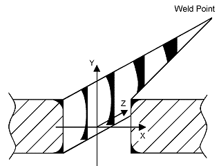To find a solution to this weld problem, or at least reduce it, we study parameters influencing the temperature distribution across the weld. In our first paper [1] we examined both development of temperature distribution in the x – y plane between coil and weld point (see figure 1) and the final distribution at the apex. In this paper we focus on the last stage and present isothermal lines for the final weld (before cooling takes place). The parameters involved in this study are Vee angle, weld speed and frequency. In addition, we investigate the impact of spring back for one given set of these three parameters.

Description of the model

An analytical approach to a solution of the problem is complicated. This is due to the three-dimensional nature of the electromagnetic field distribution for the tube welding setup. Computer aided numerical calculations based on a simplified two-dimensional model give us the capability of studying the problem. Calculations are carried out with the commercially available software Flux 2D. Assumptions made in the 2D model must be kept in mind when the results are analyzed.

The use of a 2D model can be justified, according to the following assumptions (a more thorough discussion on this can be found in [1]):

Figure 1. Weld Vee geometry with co-ordinate axis

• The Vee current's main component is in direction of the weld point (z direction); see figure 1.
• The model can be limited to a few thermal penetration depths into the tube wall (x direction) and the tube's curvature can be neglected.
• The Vee walls are parallel during the calculation
• The impeder has no influence on the local field and current distribution in the Vee.

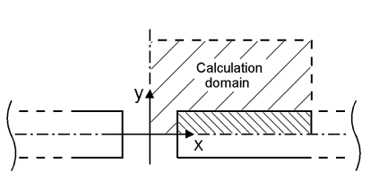
These simplifications result in symmetric current distributions on both sides of the tube wall centerline (x axis) and the vertical centerline in the weld Vee (y axis). Hence, the calculation domain can be reduced to one quarter of the Vee cross-section (see figure 2). Results are presented in this paper in figures displaying only one quarter of the actual geometry.

Figure 2. Cross-section of weld Vee

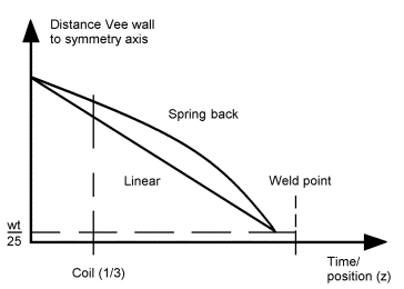
The mechanical setup of a tube welding line will determine if the movement of the strip edges towards each other is linear or not. We have concentrated our work on a setup where the movement is linear, but also looked at a phenomenon called spring back, shown in figure 3. For numerical reasons the movement is stopped when the distance between the tube wall and the symmetry axis is at 1/25 of the wall thickness.

Figure 3. Distance between Vee wall and symmetry axis vs. time

Material properties

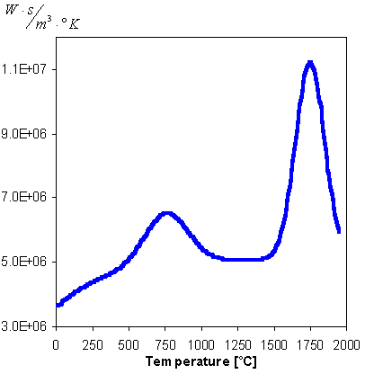
For metal strip material in our calculations we have used low-carbon steel, one of the most common materials in tube and pipe production. Low carbon steel has highly non-linear material properties. Saturation curves and rapid changes in properties at Curie temperature present a considerable problem for numerical calculations. These changes in material properties as a function of temperature have to be smoothened somewhat.

Specific heat is an example of this. At Curie temperature the material goes through a phase transformation that consumes energy, represented by a Gaussian distribution. Melting steel requires a lot of energy. In reality, this takes place in a short temperature interval. We have equaled this by another Gaussian distribution; see figure 4. As a consequence, the temperature continues to rise slowly through this interval, as opposed to being more or less constant until enough energy is absorbed to melt the steel. Using this approximation, however, makes it easier to determine how far the melting has proceeded. Temperatures above melting temperature have little practical meaning since the metal in this case will drop onto the impeder, or be thrown away by the current forces. In any case this would alter the geometry of the strip edge corners, which is not possible to simulate with this software.

Figure 4. Specific heat vs. temperature

Results

The minimum temperature required in the cross-sectional center of the tube, to avoid cold weld condition, is a function of the applied weld roll pressure. To compare the different temperature distributions, we must have a reference point. In this case, we use temperature of 1250º C in the center point (x=y=0). The current is tuned in order to get the required reference temperature. Wall thickness is 12.7 mm (0.5") in all simulations.

Simulations are carried out for three Vee angles, two mill speeds and three frequencies. Table 1 shows the calculations performed (x). In addition, one setup with 200 kHz, 14.6 m/min and 3° Vee angle with spring back has been investigated.

We present a majority of the results as isothermal lines at the weld point. Throughout the paper, we use the temperatures at lines one through nine as listed in Table 2. The temperature will not rise above the melting temperature until melting is completed. Melting alters the geometry of the tube wall and consequently influences the power distribution. The model's limitation must be kept in mind when studying the results. It is our intention to describe the parameters' influences on the temperature distribution, and not what occurs during melting.

Angle	Mill speed		Vee power	Vee voltage
°	m/min	mm	%	%
100 kHz
3	14.6	0.85	108	66
6	14.6	0.83	120	98
3	29.2	0.71	170	82
200 kHz
3	14.6	0.70	100	100
3 SB	14.6	0.69	105	115
4.5	14.6	0.68	107	128
6	14.6	0.67	112	153
3	29.2	0.59	157	121
6	29.2	0.56	179	192
300 kHz
3	14.6	0.63	96	182
6	14.6	0.59	109	201
3	29.2	0.52	152	160

To compare the setups, we have calculated the cross-sections of molten and partly molten material in the isothermal plots. In each figure we have indicated the sizes in percentage of the cross-sections for a reference setup (200 kHz, 3° Vee angle and 14.6 m/min mill speed).

Figure 5 shows the isothermal plots of upper half the tube wall cross-section for different 200 kHz setups. An increase in Vee angle from 3° to 6° increases the cross-section and amount of molten material (above 1725 °C) about three times at low speed and two times at high speed. The amount of partly molten material (above 1550 °C) increases approximately 50 % for both mill speeds.

Temperature distribution along the tube wall centerline (x-axis) is mainly affected by speed and, hence, heating time. An increase in angle and speed results in more heating of the tube wall corners. The result is a more pronounced hourglass shaped heated zone. This effect is most evident in figure 5d, with the combination of high-speed and wide angle.

Figure 6 displays the temperature distributions for 100 and 300 kHz. There are no big differences in cross-sections regarding partly molten material for these two frequencies. There is, however, a distinct difference in the amount of molten material.

References

1. J.I. Asperheim, B. Grande, L. Markegård, J.E. Buser, P. Lombard, "Temperature distribution in the cross-section of the weld Vee", Tube Int., November 1998
2. P.F. Scott, W. Smith, "The key parameters of high frequency welding", Tube Int., March 1996
3. FLUX2D user's guide, version 7.4, CEDRAT, 1999
For further information or a demo-version please contact:
Elva Induksjon as
- Addr: PO Box 760, N-3701 SKIEN, NORWAY
- Tel: +47 35 50 60 00
- Fax: +47 35 50 60 10
- WWW: http://www.efd-induction.com
- Email.
An authorization has been granted for TubeNet to publish this article
email: info@tubenet.org
Copyright © Juha Haapala. All rights reserved.